The right index on the right column, or columns, is the basis on which query tuning begins. On the other hand, a missing index or an index placed on the wrong column or columns, can be the basis for all performance problems starting with basic data access, continuing through joins, and ending in filtering clauses. For these reasons, it is extremely important for everyone – not just the DBA – to understand the different indexing techniques that can be used to optimize the database design.

The Benefits of Index in SQL Server

One of the best ways to reduce disk I/O and logical reads is to use an index,. An index allows SQL Server to find data in a table without scanning the entire table. An index in a database is analogous to an index in a book. SQL Server has to be able to find data, even when no index is present on a table. When no clustered index is present to establish a storage order for the data , the storage engine will simply read through the entire table to find what it needs. A table without a clustered index is called a heap table. A heap table is just a crude stack of data with a row identifier as a pointer to the storage location. This data is not ordered or searchable except by walking through the data, row-by-row, in a process called a scan. When a clustered index is placed on a table, the key values of the index establish an order for the data. Further with a clustered index, the data is stored with the index so that the data itself is now ordered. When a clustered index is present, the pointer on the non-clustered index consists of the values that define the clustered index. This is a big part of what makes indexes so important.

The non-clustered index usually does not contain all the columns of the table; therefore, a page will be able to store more rows of a non-clustered index than rows of the table itself, which contains all the columns. Consequently, SQL Server will be able to red more values for a column from a page representing a non-clustered index on the column than from a page representing the table that contain the column. Another benefit of the non-clustered index is that, because it is in a separate structure from the data table, it can be put in a different filegroup, with a different I/O path.

Initial Layout of 27 Rows

Ordered Layout of 27 Rows

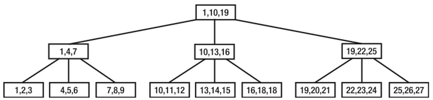
B-Tree Layout of 27 Rows

Indexes store their information in a B-tree structure, so the number of reads required to find a particular row is minimized. The above example shows the benefit of a B-Tree structure. Consider the single column table with 27 rows in a random order and only 3 rows per leaf page, suppose that layout of the rows in the pages is as shown in ‘Initial Layout of 27 Rows’ figure. To search the row for the column value of 5, SQL Server has to scan all the rows and the pages, since even the last row in the last page may have the value 5. because the number of reads depends on the number of pages accessed, nine read operations have to be performed without an index on the column. This content can be ordered by creating an index on the column, with the resultant layout of the rows and pages shown in ‘Ordered Layout of 27 rows’. Indexing the column arranges the content in a sorted fashion. This allows SQL Server to determine the possible value for a row position in the column with resect to the value of another row position in the column.

A B-tree consists of a starting node (or page) called a root node with branch nodes (or pages) growing out of it (or linked to it). All keys are stored in the leaves. Contained in each interior node (above the leaf nodes) are pointers to its branch nodes and values representing the smallest value found in the branch node. Keys are kept in sorted order within each node. B-trees use a balanced tree structure for efficient record retrieval—a B-tree is balanced when the leaf nodes are all at the same level from the root node. For example, creating an index on the preceding content will generate the balanced B-tree structure shown in ‘B-Tree Layout 27 Rows’. The B-Tree algorithm minimizes the number of pages to be accessed to locate a desired key, thereby speeding up the data access process. 

The Index Overhead

The performance benefit of indexes come at a cost. Tables with indexes require more storage and memory space for the index pages in addition to the data pages of the table. Data manipulation queries (Insert, Update, and Delete statements, or the CUD) can take longer, and more processing time is required to maintain the indexes of constantly changing tables. This is because, unlike a SELECT statement, data manipulation queries modify the data content of a table. If an INSERT statement adds a row to the table, then it also has to add a row in the index structure. If the index is a clustered index, the overhead is greater still, because the row has to be added to the data pages themselves in the right order, which may require other data rows to be repositioned below the entry position  of the new row. The UPDATE and DELETE data manipulation queries change the index pages in a similar manner.

When designing indexes, you will be operating from two different points of view: the existing system, already in production, where you need to measure the overall impact of an index, and the tactical approach where all you worry about is the immediate benefits of an index, usually when initially designing a system. When you have to deal with the existing system, you should ensure that the performance benefits of an index outweigh the extra cost in processing resources.

When you are focused exclusively on the immediate benefits of an index, SQL Server supplies a series of dynamic management views that provide detailed information about the performance of indexes.

• Sys.dm_db_index_operational_stats
• Sys.dm_db_index_usage_stats

To understand the overhead cost of an index on data manipulation queries, consider the above example.

Create Table TempTable ( C1 int , C2 int, C3 char(50));
Go
Select Top 10000 Identity(int,1,1) as n
Into #Temp From master.dbo.syscolumns;
Go
Insert Into TempTable(C1,C2,C3) Select n, n, ’C3’ From #Temp;
Go
Set Statistics IO on;
Go
Update TempTable Set C1 = 1, C2 = 1 Where C1 = 1;

The number of logical reads reported by ‘Set Statistics IO’ is as follows:

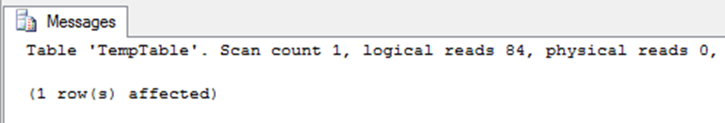
Table ‘TempTable’, Scan count 1, logical reads 8, physical reads 0

Even though it is true that the amount of overhead required to maintain indexes increases for data manipulation queries, be aware that SQL Server must first find a row before it can update or delete it; therefore, indexes can be helpful for UPDATE and DELETE statements with complex WHERE clauses as well. The increased efficiency in using the index to locate a row usually offsets the extra overhead needed to update the indexes, unless the table has a lot of indexes.

 

Create Clustered Index IX1 on TempTable (C1);
Go
Update TempTable Set C1 = 1, C2 = 1 Where C1 = 1;

Go
Create Index IX2 on TempTable(C2);
Go
Update TempTable Set C1 = 1, C2 = 1 Where C2 = 1;

To understand how an index can benefit even data modification queries, lets build on the example. Create another index on table ‘TempTable’ as above example, this time, we create the index on column C2 referred to in the WHERE clause of the UPDATE statement.

Create Index IX2 On TempTable(C2);

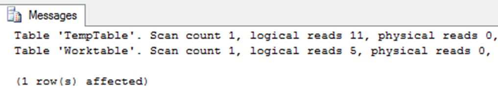
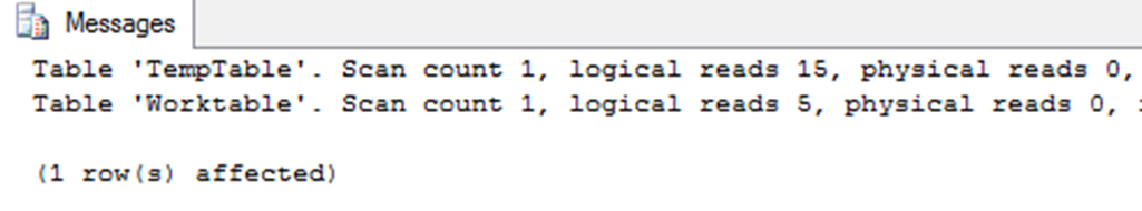
After adding this new index, run the UPDATE command one more time, and you will see the number of logical reads for this UPDATE statement decreases from 84 to 20 which is combination of 15 for TempTable and 5 for Worktable.

A worktable is a temporary table used internally by SQL Server to process the intermediate results of a query. Worktables are created in the tempdb database and are dropped automatically after query execution.

Index Design Recommendations 

When a query is submitted to SQL Server, the optimizer tries to find the best data access mechanism for every table referred to in the query. Here is how it does this:

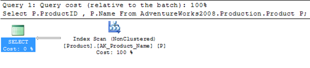
Select P.ProductID , P.Name  From Production.Product;

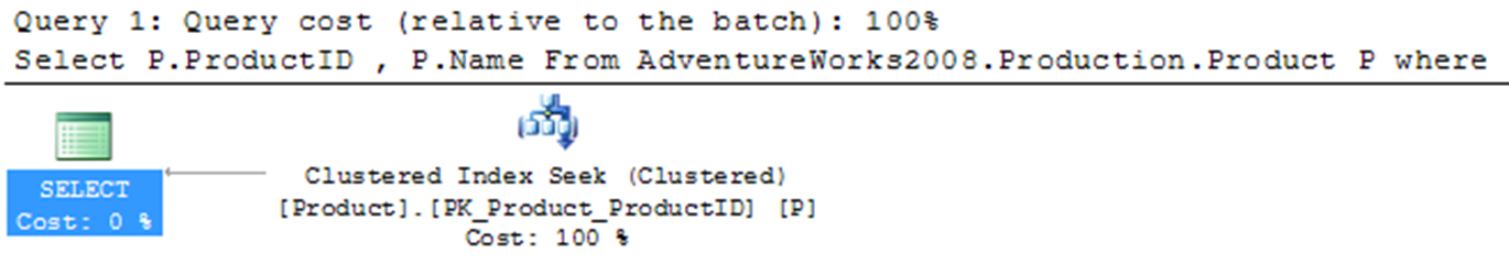
Select P.ProductID , P.Name From Production.Product
Where P.ProductID = 726;

1. Optimizer identifies the columns included in the WHERE clause and the JOIN criteria.
2. Optimizer then examines indexes on those columns.
3. Optimizer assesses the usefulness of each index by determining the selectivity of the clause from statistics maintained on the index.
4. Finally, estimates the least costly method of retrieving the qualifying rows, based on the information gathered in the previous steps.
5. To understand the significance of a WHERE clause column in a query, lets consider the above example, the query optimizer performs a non-clustered index scan to read the rows as the first figure. With the WHERE clause in place, the optimizer examines the WHERE clause column ProductId, identifies the availability of the Index ‘PK_Product_ProductID’ and decides to use that index on column ProductId, and second figure.
6. The behavior of the query optimizer shows that the WHERE clause column helps the optimizer choose an optimal indexing operation for a query. This is also applicable for a column used in the join criteria between two tables. The optimizer looks for the indexes on the WHERE clause columns or the join criterion column and if available, considers using the index to retrieve the rows from the table. The query optimizer considers index(es) on the WHERE clause column(s) and the join criteria column(s) while executing a query. Therefore, having indexes on the frequently used columns in the WHERE clause and join criteria of a SQL query helps optimizer avoid scanning a base table.

You can create indexes on a combination of columns in a table. For the best performance, use as few columns in an index as you can. You should also avoid very wide data type columns in an index. Columns with string data types sometimes can be quite wide as can binary; unless they are absolutely necessary, minimize the use of wide data type columns with large sizes in an index.

Use Narrow Index

A narrow index can accommodate more rows in an 8KB index page than a wide index. This has the following effects:

• Reduces I/O.
• Makes database caching more effective, because SQL Server can cache fewer index pages, consequently reducing the logical reads required for the index pages in the memory.
• Reduces the storage space for the database.

To understand how a narrow index can reduce the number of logical reads, create a test table with 20 rows and an index on it.

CREATE TABLE TESTTABLE (C1 INT, C2 INT);
WITH NUMS AS (
SELECT 1 AS N
UNION ALL  
SELECT N + 1 FROM NUMS
WHERE N < 20)

INSERT INTO TESTTABLE (C1,C2)
SELECT N, 2 FROM NUMS;

CREATE INDEX IX1 ON TESTTABLE (C1);
/*THE DMF SYS.DM_DB_INDEX_PHYSICAL_STATS,, CONTAINS THE MORE DETAILED INFORMATION ABOUT THE STATISTICS ON THE INDEX. TO UNDERSTAND THE DISADVANTAGE OF A WIDE INDEX KEY, MODIFY THE DATA TYPE OF THE INDEXED COLUMN C1 FROM INT TO CHAR(500). */

DROP INDEX TESTTABLE.IX1;
ALTER TABLE TESTTABLE ALTER COLUMN C1 CHAR(500);
CREATE INDEX IX1 ON TESTTABLE(C1);

Creating an Index on columns with a very low range of possible values (such as gender) will not benefit performance, because the query optimizer will not be able to use the index to effectively narrow down the rows to be returned. Consider a ‘Gender’ column with only two unique values: M and F. when you execute a query with Gender column in the WHERE clause, you end up with a large number of rows from the table (assuming the distribution of M and F is even), resulting in a costly table or clustered index scan. It is always preferable to have columns in the WHERE clause with lots of unique rows (or high selectivity) to limit the number of rows accessed. You should create an index on those column(s) to help the optimizer access a small result set.

Furthermore, while creating an index on multiple columns, which is also referred to as a composite index, column order matters. In some cases, using the most selective column first will help filter the index rows more efficiently.

Examine the Column Value Uniqueness

From this, you can see that it is important to know the selectivity of a column before  creating an index on it. You can find this by executing a query like this one; just substitute the table and column name.

SELECT COUNT (DISTINCT GENDER) AS DISTINCTVALUES,
COUNT (GENDER) AS NUMBEROFROWS,
(CAST(COUNT(DISTINCT GENDER) AS DECIMAL) / CAST ( COUNT(GENDER) AS DECIMAL)) AS SELECTIVITY
FROM HUMANRESOURCES.EMPLOYEE;

The column with the higher number of unique values can be the best candidate for indexing when referred to in a WHERE clause or a join criterion.

Examine the Column Data Type 

The data type of an index matters. For example, an index search on integer keys is very fast because of the small size and easy arithmetic manipulation of the INTEGER (or INT) data type. You can also use other variations of integer data types (BigInt, SmallInt and TinyInt) for index columns, whereas string data types require a string match operation, which is usually costlier than an integer match operation.

Suppose you want to create an index on one column and you have two candidate columns, one with an INTEGER data type and the other with a CHAR(4) data type. Even though the size of both data types is 4 bytes in Sql server, You will still prefer the INTEGER data index. Look at arithmetic operations as an example. The value 1 in the CHAR94) data type is actually stored as 1 followed by three spaces, a combination of the following four bytes: 0x35,0x20,0x20 and 0x20. the CPU does not understand how to perform arithmetic operations on this data, and therefore it converts to an integer data type before the arithmetic operations, whereas the value 1 in an INTEGER data type is saved as 0x00000001. The CPU can easily perform arithmetic operations on this data.

Of course, most of the time, you won’t have the simple choice between identically sized data types, allowing you to choose the more optimal type. Keep this information in mind when designing and building your indexes.

Consider Column Order

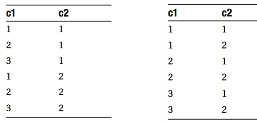
An index key is sorted on the first column of the index and then sub-sorted on the next column within each value of the previous column. The first column in a compound index is frequently referred to as the ‘Leading Edge’ of the index. For example, consider the ‘Heap Table’ figure. If a composite index is created on the columns (C1, C2) then the index will be ordered as shown in ‘Composite Index’ figure.

Create Nonclustered Index NCIX_Address on Person.Address (City, PostalCode);
Go
Select City, PostalCode from Person.Address
Where City = ‘Walla Walla’;

To understand the importance of column ordering in an index, consider the above example. In the ‘Person.Address’ table, there is a column for ‘City’ and another for ‘PostalCode’. Create a temporary index on the table like above.

A simple SELECT statement run against the table that will use this new index will look something above I/O and execution time from statistics.

Select * from Person.Address with (Index(NCIX_Address))
Where City = ‘Walla Walla’and PostalCode = ‘WA3 7BH’;

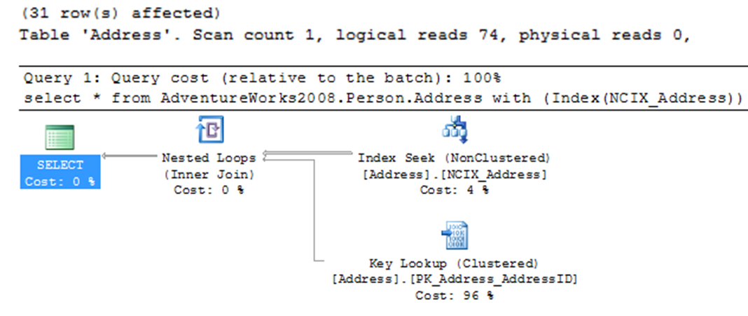
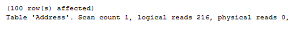
Executing this query will return the same 31 rows as the previous query, resulting in the following:

Select City, PostalCode from Person.Address with (Index(NCIX_Address))
Where City = ‘Walla Walla’and PostalCode = ‘WA3 7BH’;

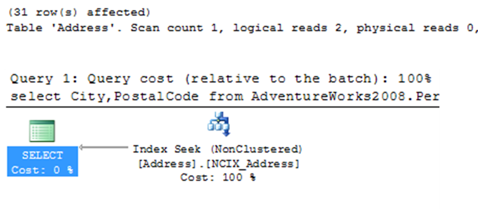
Table ‘Address’. Scan count 1, Logical reads 2

The radical changes in I/O and execution plan represent the real use of a compound index, the covering index. This is covered in detail in the section “Covering Indexes” later in the module.

Clustered Index in SQL Server

In SQL Server, you have two main index types: clustered and non-clustered. Both types have a B-tree and Columnstore structures (Columnstore indexes are discussed in ‘SQL Server DW-BI Performance Tuning Course'. The main difference between the two types is that the leaf pages in a clustered index are the data pages of the table and are therefore in the same order as the data to which they point. This means that the clustered index is the table. As you proceed, you will see that the difference at the leaf level between the two index types becomes very important when determining the type of index to use.

The leaf pages of a clustered index and the data pages of the table the index is on are one and the same. Because of this, table rows are physically sorted on the clustered index column, and since there can be only one physical order of the table data, a table can have only one clustered index.

Clustered Index Recommendations

The relationship between a clustered index and a non-clustered index imposes some considerations on the clustered index, which are explained in the sections that follow:

• Create Clustered Index First: Since all non-clustered indexes hold clustered index keys within their index rows, the order of non-clustered and clustered index creation is very important. For example, if the non-clustered indexes are built before the clustered index is created, then the non-clustered index row locator will contain a pointer to the corresponding RID of the table. Creating the clustered index later will modify all the non-clustered indexes to contain clustered index keys as the new row locator value. This effectively rebuilds all the non-clustered indexes. For the best performance, I recommend that you create the clustered index before you create any non-clustered index. This allows the non-clustered indexes to have their row locator set to the clustered index keys at the time of creation. This does not have any effect on the final performance, but rebuilding the indexes may be quite a large job.
• Keep the Index Key Narrow: Since all non-clustered indexes hold the clustered keys as their row locator, for the best performance keep the overall byte size of the clustered index as small as possible. If you create a wide clustered index, say CHAR(500), this will add 500 bytes to every non-clustered index. Thus, keep the number of columns in the clustered index to a minimum, and carefully consider the byte size of each column to be included in the clustered index. A column of the INTEGER data type usually makes a good candidate for a clustered index, whereas a string data type column will be a less-than-optimal choice.
• Rebuild the Clustered Index in single Step: Because of the dependency of non-clustered indexes on the clustered index, rebuilding the clustered index as separate DROP INDED and CREATE INDEX statements causes all the non-clustered indexes to be rebuild twice. To avoid this, use the DROP_EXISTING clause of the CREATE INDEX statement to rebuild the clustered index in a single atomic step. Similarity, you can also use the DROP_EXISTING clause with a non-clustered index.
• Create Clustered Index with Preorder Sort: Clustered Indexes are particularly efficient when the data retrieval needs to be sorted. If you create a clustered index on the column or columns that you may need to sort by, then the rows will be physically stored in that order, eliminating the overhead of sorting the data after it is retrieved.
• Do not Create Clustered Index on Frequently Updatable Column: If the clustered index columns are frequently updated, this will cause the row locator of all the non-clustered indexes to be updated accordingly, significantly increasing the cost of the relevant action queries. This is also affects database concurrency by blocking all other queries referring to the same part of the table and the non-clustered indexes during that period.   Therefore, avoid creating a clustered index on columns that are highly updatable.
• Do not Use Wide Keys: Since all non-clustered indexes hold the clustered keys as their row locator, for performance reasons you should avoid creating a clustered index on a very wide column (or columns) or on too many columns. As explained in the preceding section, a clustered index must be as narrow as possible.
• Prevent Too Many Concurrent Inserts in Sequential Order: If you want to add many new rows concurrently, then it may be better for performance to distribute them across the data pages of the table. However, if you add all the rows in the same order as that imposed by the clustered index, then all the inserts will be attempted on the last page of the table. This may cause a huge “hot spot” on the corresponding sector of the disk. To avoid this disk hot spot, you should not arrange the data rows in the same order as their physical locations. The inserts can be randomized throughout the table by creating a clustered index on another column that does not arrange the rows in the same order as that of the new rows. This is an issue only with a large number of simultaneous inserts.

There is a caveat to this recommendation. Allowing inserts on the bottom of the table prevents page splits on the intermediate pages that are required to accommodate the new rows in those pages. If the number of concurrent inserts is low, then ordering the data rows (using a clustered index) in the order of the new rows will prevent intermediate page splits. However, if the disk hot spot becomes a performance bottleneck, then new rows can be accommodated in intermediate pages without causing page splits by reducing the fill factor of the table. In addition, the “hot” pages will be in memory, which also benefits performance.

Non-Clustered Index in SQL Server

A non-clustered index does not affect the order of the data in the table pages, because the leaf pages of a non-clustered index and the data pages of the table are separate. A pointer (the row locator) is required to navigate from an index row to the data row. As you learned in the earlier “Clustered Index” section, the structure of the row locator depends on whether the data pages are stored in a heap or a clustered index. For a heap, the row locator is a pointer to the RID for the data row; for a table with a clustered index, the row locator is the clustered index key.

The row locator value of the non-clustered indexes continues to have the same clustered index value, even when the clustered index rows are physically relocated. To optimize this maintenance cost, SQL Server adds a pointer to the old data page to point to the new data page after a page split, instead of updating the row locator of all the relevant non-clustered indexes. Although this reduces the maintenance cost of the non-clustered indexes, it increases the navigation cost from the non-clustered index row to the data row, since an extra link I added between the old data page and the new data page. Therefore, having a clustered index as the row locator decreases this overhead associated with the non-clustered index.

When a query requests column that are not part of the non-clustered index chosen by the optimizer, a lookup is required. This may be a key lookup when going against a clustered index or an RID lookup when performed against a heap. The common term for these lookups comes from the old definition name, bookmark lookup. The lookup fetches the corresponding data row from the table by following the row locator value from the index row requiring a logical read on the data page besides the logical read on the index page. However, if all the columns require by the query are available in the index itself, then access to the data page is not required. This is known as a covering index.

Non-Clustered Index Recommendations

Since a table can have only one clustered index, you can use the flexibility of multiple non-clustered indexes to help improve performance. I explain the factors that decide the use of a non-clustered index in the following sections.

A non-clustered index is most useful when all you want to do is retrieve a small number of rows from a large table. As the number of rows to be retrieved increases, the overhead cost of the bookmark lookup rises proportionately. To retrieve a small number of rows from a table, the indexed column should have a very high selectivity.

Furthermore, there will be indexing requirements that won’t be suitable for a clustered index, as explained in the “Clustered Indexes” section:

• Frequently Updatable Columns
• Wide Keys

In these cases, you can use a non-clustered index, since, unlike a clustered index, it doesn’t affect other indexes in the table. A non-clustered index on a frequently updatable column is not as costly as having a clustered index on that column.

Non-clustered indexes are not suitable for queries that retrieve a large number of rows, such queries better served with a clustered index, which does not require a separate bookmark lookup to retrieve a data row. If your requirement is to retrieve a large result set from a table, then having a non-clustered index on the filter criterion (or the join criterion) column will not be useful unless you use a special type of non-clustered index called a covering index. I describe this index type in detail later in the module.

Benefits of Clustered Over Non-Clustered Index

 

The main considerations in choosing between a clustered and a non-clustered index are as follows:

• Number of Rows to be Retrieved.
• Data-Ordering Requirement
• Index Key Width
• Column Update Frequency
• Bookmark Cost
• Any Disk Hot Spots

When deciding upon type of index on a table with no indexes, the clustered index is usually the preferred choice. Because the index page and the data pages are the same, the clustered index doesn’t have to jump from the index row to the base row as required in the case of a non-clustered index.

To understand how a clustered index can outperform a non-clustered index in most circumstances, even in retrieving small number of rows, we create a test table with a high selectivity for one column:

CREATE TABLE TEMPTABLE (C1 INT , C2 INT);
GO
SELECT TOP 10000 IDENTITY(INT,1,1) AS N
INTO #NUM
FROM MASTER.DBO.SYSCOLUMNS;
GO
INSERT INTO TEMPTABLE(C1,C2) SELECT N,N FROM #NUM;

The following SELECT statement fetches only 1 out of 10,000 rows from the table:

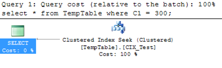
SELECT * FROM TEMPTABLE WHERE C1 = 300;

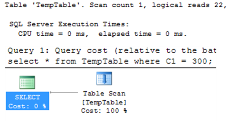
With the graphical execution plan shown in above figure and the output of SET STATISTICS IO as follows:

Table ‘TempTable’. Scan count 1, logical reads 22

Considering the small size of result set retrieved by the preceding SELECT statement, a non-clustered column on C1 can be a good choice:

CREATE NONCLUSTERED INDEX NCIX ON TEMPTABLE (C1);

You can run the same SELECT command again, since retrieving a small number of rows through a non-clustered index is more economical than a table scan, the optimizer used the non-clustered index on column C1 as shown in above figure. The number of logical reads reported by SET STATISTICS IO is as follows:

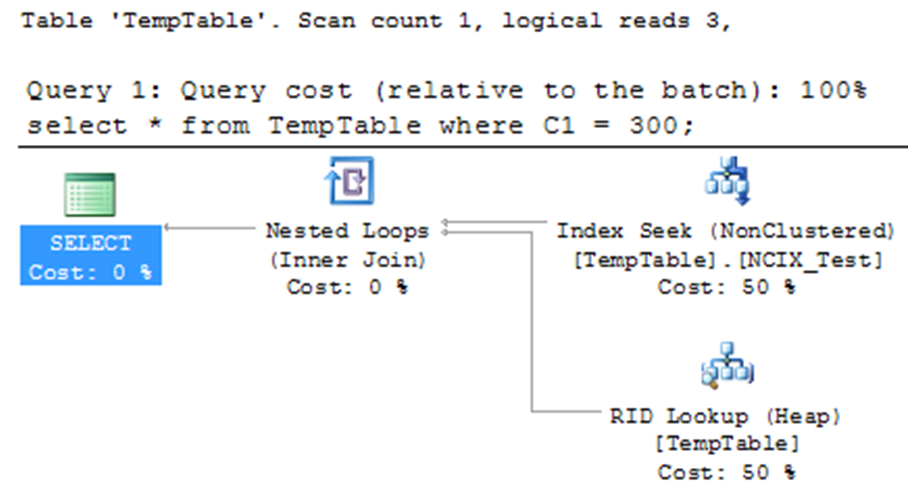
Table ‘TempTable’. Scan counts 1, logical reads 3

Even though retrieving a small result set using a column with high selectivity is a good pointer toward creating a non-clustered index on the column, a clustered index on the same column can be equally beneficial or even better. To evaluate how the clustered index can be more beneficial than the non-clustered index, create a clustered index on the same column:

CREATE CLUSTERED INDEX CIX ON TEMPTABLE(C1);

Run the same SELECT command again. From the resultant execution plan (see above figure) of the preceding SELECT statement, you can see that the optimizer used the clustered index (instead of the non-clustered index) even for a small result set. The number of logical reads for the SELECT statement decreased from three to two as above figure.

Even though a clustered index can outperform a non-clustered index in many instances of data retrieval, a table can have only one clustered index. Therefore, reserve the clustered index for a situation in which it can be of the greatest benefit.

Benefits of Non-Clustered Over Clustered Index

As you learned in the previous section, a non-clustered index is preferred over a clustered index in the following situations:

• When the index key size is large.
• To avoid the overhead cost associated with a clustered index since rebuilding the clustered index rebuilds all the non-clustered indexes of the table.
• To resolve blocking by a database reader work on the pages of a non-clustered index, while a database writer modifies other columns in the data pages.
• When all the columns referred to by a query ca be safely accommodated in the non-clustered index itself, as explained in this module.

As already established, the data-retrieval performance when using a non-clustered index is generally poorer than that when using a clustered index, because of the cost associated in jumping from the non-clustered index rows to the data rows in the base table. In cases where the jump to the data rows is not required, the performance of a non-clustered index should be just as good as or even better than a clustered index. This is possible if the non-clustered index key includes all the columns required from the table.

To understand the situation where a non-clustered index can outperform a clustered index, consider the following example. Assume for our purposes that you need to examine the credit cards that are ‘Distinguish’.

SELECT CARDTYPE, CARDNUMBER, EXPMONTH
FROM SALES.CREDITCARD
WHERE CARDTYPE = ‘DISTINGUISH’;

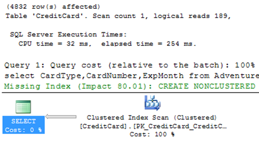
The following are the I/O results and the above figure is the execution plan:

Table ‘CreditCards’. Scan counts 1, Logical reads 189 

The clustered index is on the primary key, and although most access against the table may be through that key, making the index useful, the cluster in this instance is just not performing in the way you need. Although you could expand the definition of the index to include all the other columns in the query, they’re not really needed to make the cluster function, and they would interfere with the operation of the primary key. In this instance, creating a different index is in order:

CREATE NONCLUSTERED INDEX NCIX ON SALES.CREDITCARD (CARDTYPE, CARDNUMBER, EXPMONTH);

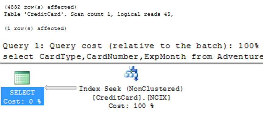
Now when the query is run again, this is the I/O result and execution plan as above figure:

Table ‘CreditCards’. Scan counts 1, logical reads 45

Covering Indexes in SQL Server

A covering index is a non-clustered index built upon all the columns required to satisfy a SQL query without going to the base table. If a query encounters an index and does not need to refer to the underlying data table at all, then the index can be considered a covering index.

A covering index is a useful technique for reducing the number of logical reads of a query. Adding columns using the INCLUDE statement makes this functionality easier to achieve without adding to the number of columns in an index or the size of the index key since the included columns are stored only at the leaf level of the index.

The INCLUDE is best used in the following cases:

• You do not want to increase the size of the index keys, but you still want to make the index a covering index.
• You are indexing a data type that cannot be indexed (except text, text and image)
• You have already exceeded the maximum number of key columns for an index.

The covering index physically organizes the data of all the indexed columns in a sequential order. Thus, from a disk IO perspective, a covering index that does not use INCLUDE columns becomes a clustered index for all queries satisfied completely by the columns in the covering index. If the result set of a query requires a sorted output, then the covering index can be used to physically maintain the column data in the same order s required by the result set, it can then be used in the same way as a clustered index for sorted output.

To take advantage of covering indexes, be careful with the column list in SELECT statements. Use as few columns as possible to keep the index key size small for the covering indexes. Add columns using the INCLUDE statement in places where it makes sense. Since a covering index includes all columns used in a query, it has a tendency to be very wide, increasing the maintenance cost of the covering indexes. You must balance the maintenance cost with the performance gain that the covering index brings. If the number of bytes from all the columns in the index is small compared to the number of bytes in a single data row of that table and you are certain the query taking advantage of the covered index will be executed frequently, then it may be beneficial to use a covering index.

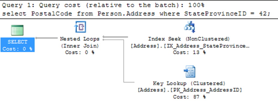
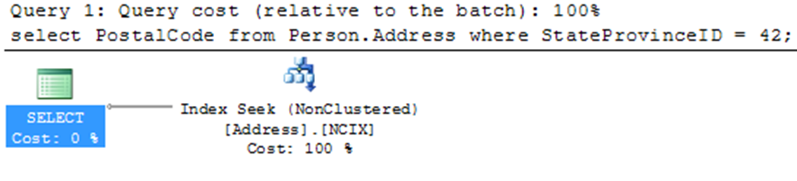
For example, in the following SELECT statement, irrespective of where the columns are referred, all the columns (StateProvinceId and PostalCode) should be included in the non-clustered index to cover the query fully:

SELECT POSTALCODE
FROM PERSON.ADDRESS
WHERE STATEPROVINCEID = 42;

Then all the required data for the query can be obtained from the non-clustered index page, without accessing the data page.

Here you have a classic bookmark lookup with the Key Lookup operator pulling the PostalCode data from the clustered index and joining it with the Index Seek operator against the IX_Address_StateProvinceId index.

Although you can re-create the index with both key columns, another way to make an index a covering index is to use the new INCLUDE operator. This stores data with the index without changing the structure of the index itself. Use the following to re-create the index:

CREATE NONCLUSTERED INDEX NCIX ON PERSON.ADDRESS (STATEPROVINCEID ASC) INCLUDE (POSTALCODE);

If you rerun the query, the execution plan change. 

Index Intersection in SQL Server

If a table has multiple indexes, then SQL Server can use multiple indexes to execute a query. SQL Server can take advantage of multiple indexes, selecting small subsets of data based on each index and then performing an intersection of the two subsets. SQL Server can exploit multiple indexes on a table and then employ a join algorithm to obtain the index intersection between the two subsets.

In the following SELECT statement, for the WHERE clause columns the tale has a non-clustered index on the SalesPersonID column, but it has no index on the OrderDate column:

SELECT SOH.*
FROM SALES.SALESORDERHEADER SOH
WHERE SOH.SALESPERSONID = 276 AND
SOH.ORDERDATE BETWEEN'01-01-2000'AND '01-01-2002';

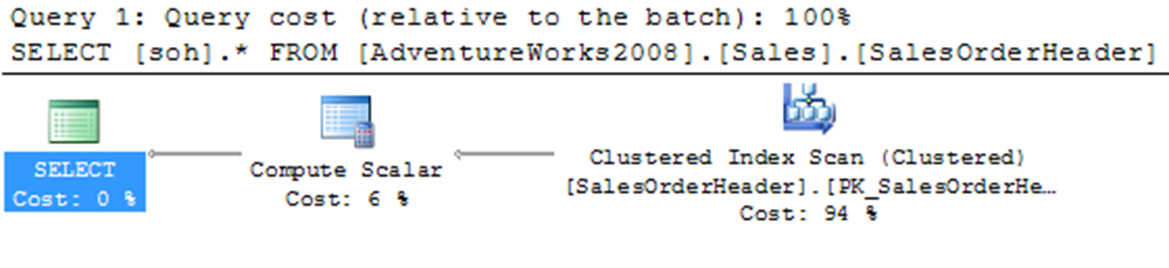
As you can see, the optimizer didn’t use the non-clustered index on the SalesPersonID column. Since the value of the OrderDate column is also required, the optimizer chose the clustered index to fetch the value of all the referred columns. To improve the performance of the query, the OrderDate column can be added to the non-clustered index on the SalesPersonID column or defined as an include column on the same index. But in this real-world scenario, you may have to consider the following while modifying an existing index:

• It may not be permissible to modify an existing index for various reasons.
• The existing non-clustered index key may be already quite wide.
• The cost of the queries using the existing index will be affected by the modification.

In such cases, you can create a new non-clustered index on the OrderDate column

CREATE INDEX NCIX ON SALES.SALESORDERHEADER (ORDERDATE);

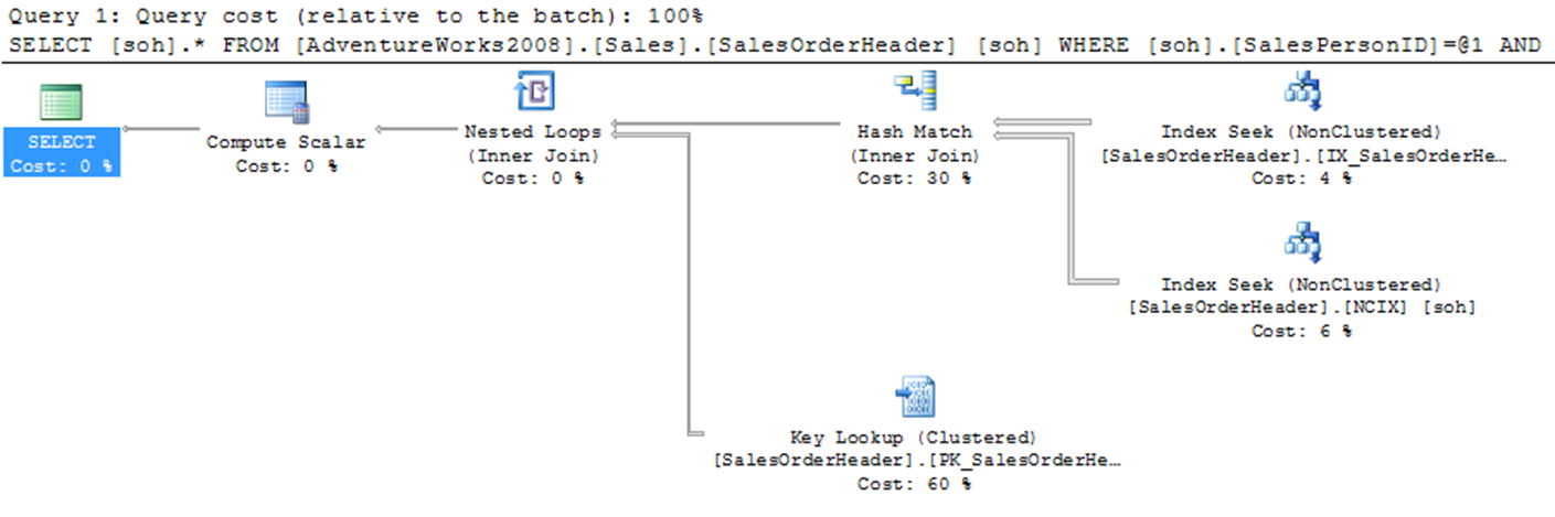
As you can see, SQL Server exploited both the non-clustered indexes as index seeks (rather than scans) and then employed an intersection algorithm to obtain the index intersection of the two subsets. It then did a Key Lookup from the resulting data to retrieve the rest of the data not included in the indexes.

To improve the performance of a query, SQL Server can use multiple indexes on a table. Therefore, instead of creating wide index keys, consider creating multiple narrow indexes. SQL Server will be able to use them together where required, and when not required, queries benefit from narrow indexes. While creating a covering index, determine whether the width of the index will be acceptable and whether using include columns will get the job done. If not, then identify the existing non-clustered indexes that include most of the columns required by the covering index. You may already have two existing non-clustered indexes that jointly serve all the columns required by the covering index. If it is possible, rearrange the column order of the existing non-clustered indexes appropriately, allowing the optimizer to consider an index intersection between the two non-clustered indexes.

At times, it is possible that you may have to create a separate non-clustered index for the following reasons:

• Reordering the columns in one of the existing indexes is not allowed.
• Some of the columns required by the covering index may not be included in the existing non-clustered indexes.
• The total number of columns in the two existing non-clustered indexes may be more than the number of columns required by the covering index.

Filtered Index in SQL Server 

A filtered index is a non-clustered index that uses a filter, basically a WHERE clause, to create a highly selective set of keys against a column or columns that may not have good selectivity otherwise. For example, a column with a large number of NULL values may be stored as a sparse column to reduce the overhead of those NULL values. Adding a filtered index to the column will allow you to have an index available on the data that is not NULL. The best way to understand this is to see it in action.
The ‘Sales.SalesOrderHeader’ table has more than 30,000 rows. Of those rows, 27,000+ have a NULL value in the PurchaseOrderNumber column and the SalesPersionID column. If you wanted to get a simple list of purchase order numbers, the query might look like this:

SELECT SOH.*
FROM SALES.SALESORDERHEADER SOH
WHERE SOH.PURCHASEORDERNUMBER LIKE 'PO%'AND SOH.SALESPERSONID IS NOT NULL;

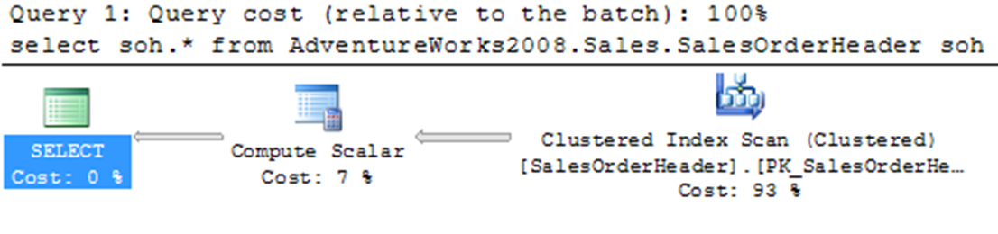
Running the query results in, as you might expect, a clustered index scan, and the following I/O and execution plan shown as above.

Table ‘SalesOrderHeader’. Scan Counts 1, Logical reads 686

To fix this, it is possible to create and adjust the index so that it filters out the NULL values, which aren’t used by the index anyway, reducing the size of the tree and therefore the amount of searching required.

CREATE INDEX NCIX ON SALES.SALESORDERHEADER (PURCHASEORDERNUMBER, SALESPERSONID)
WHERE ( PURCHASEORDERNUMBER IS NOT NULL AND SALESPERSONID IS NOT NULL);

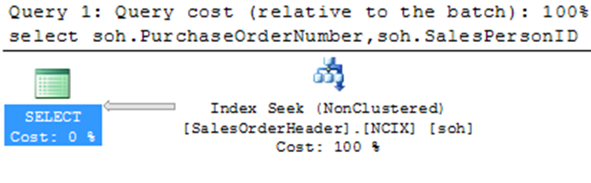
The final run of the query is visible in the above execution plan figure.

One of the first places suggested for their use is just like the previous example, eliminating NULL values from the index. You can also isolate frequently accessed sets of data with a special index so that the queries against that data perform much faster. You can use the WHERE clause to filter data in a fashion similar to creating an indexed view without the data maintenance headaches associated with indexed views by creating a filtered index that is a covering index.

Indexed Views or Materialized Views in SQL Server

A database view in SQL Server is like a virtual table that represents the output of a SELECT statement. You create a view using the CREATE VIEW statement, and you can query it exactly like a table. In general, a view doesn’t store any data—only the SELECT statement associated with it. Every time a view is queried, it further queries the underlying tables by executing its associated SELECT statement.

A database view can be materialized on the disk by creating a unique clustered index on the view. Such a view is referred to as an indexed view or a materialized view. After a unique clustered index is created on the view, the view’s result set is materialized immediately and persisted in physical storage in the database, saving the overhead of performing costly operations during query execution. After the view is materialized, multiple non-clustered indexes can be created on the indexed view.

Indexed views can produce major overhead and restrictions on an OLTP database. Some of the overheads of indexed views are as follows:

• Any change in the base table(s) has to be reflected in the indexed view.
• Any changes to a base table on which an indexed view is defined may initiate one or more changes in the non-clustered indexes of the indexed view.
• The indexed view adds to the ongoing maintenance overhead of the database.
• Additional storage is required.
• The first index on the view must be a unique clustered index.
• Non-clustered indexes on an indexed view ca be created only after the unique clustered index is created.
• The view definition must be deterministic.
• The indexed view must reference only base table in the same database, not other views.
• The indexed view may contain float columns.
• The indexed view must be a schema bound to the tables referred.

Reporting systems benefit the most from indexed views. OLTP systems with frequent writes may not be able to take advantage of the indexed views because of the increased maintenance cost associated with updating both the view and the underling base tables. The net performance improvement provided by an indexed view is the difference between the total query execution savings offered by the view and the cost of storing and maintaining the view.

Index Compression in SQL Server

Data and index compression was introduced in SQL Server 2008. Compressing an index means getting more key information onto a single page. This can led to serious performance improvements because fewer pages and fewer index levels are needed to store the index. There will be overhead in the CPU and memory as the key values in the index are compressed and decompressed, so this may not be a solution for all indexes.

By default an index will not be compressed and you have to explicitly call for the index  to be compressed when you create the index.

Consider the following Indexes as example:

CREATE NONCLUSTERED INDEX NCIX_TEST ON PERSON.ADDRESS (CITY, POSTALCODE);
GO
CREATE NONCLUSTERED INDEX NCIX_PAGE_TEST ON PERSON.ADDRESS (CITY, POSTALCODE)
WITH (DATA_COMPRESSION = PAGE);
GO
CREATE NONCLUSTERED INDEX NCIX_ROW_TEST ON PERSON.ADDRESS (CITY, POSTALCODE)
WITH (DATA_COMPRESSION = ROW);

Spatial Index in SQL Server 

As special data types and storage mechanisms are introduced to SQL Server by Microsoft, methods for indexing these special storage types are also developed. Explaining all the details possible for each of these special index types is outside the scope of the book. In the following sections, I introduce the basic concepts of each index type in order to facilitate the possibility of their use in tuning your queries.

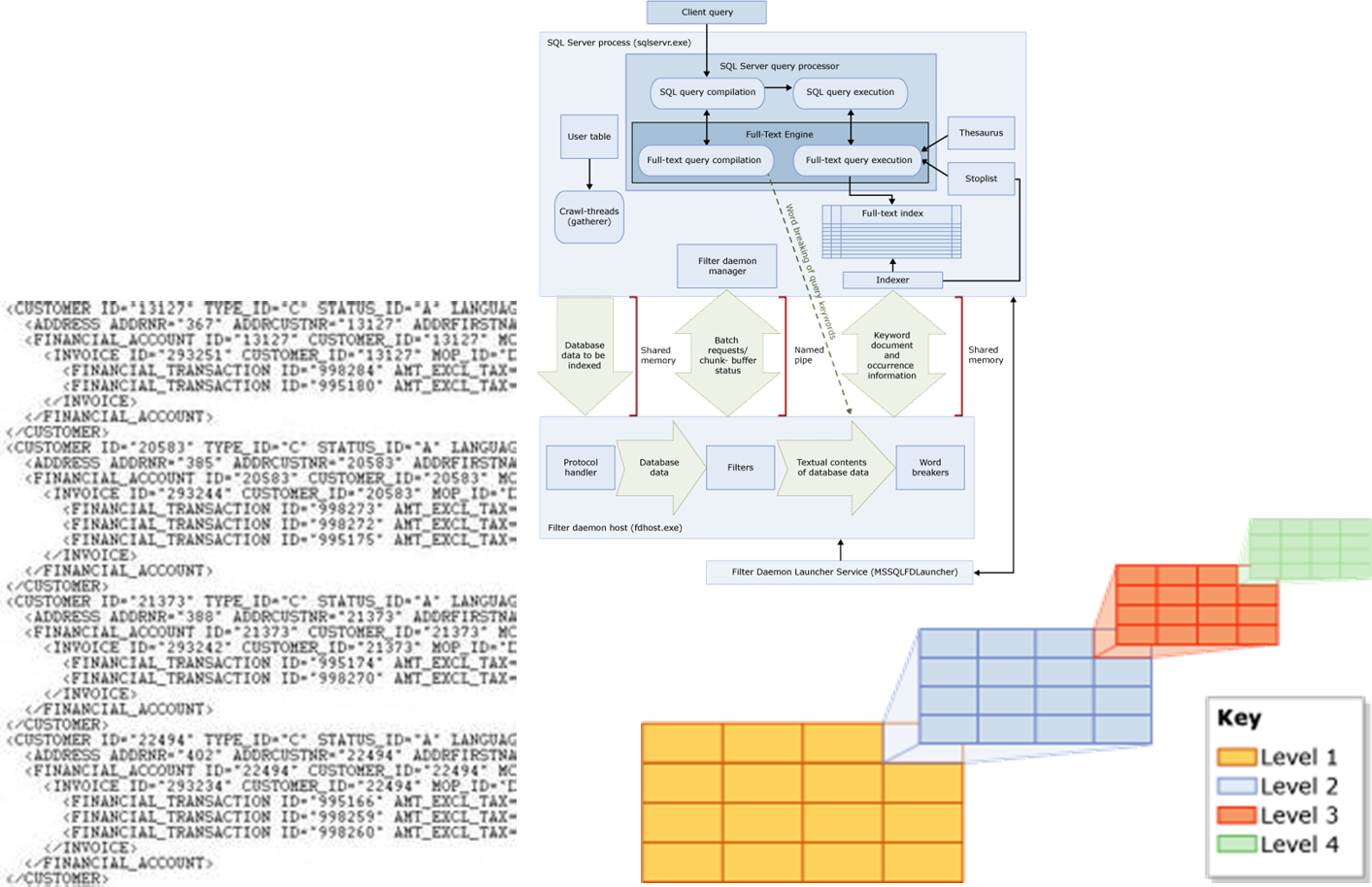
Full-Text

You can store large amounts o text in Sq server by using the MAX value in the VARCHAR, NVARCHAR, CHAR and NCHAR fields. A normal clustered or non-clustered index against these large fields would be unsupportable because a single value can far exceed the page size within an index. So, a different mechanism of indexing text is to use the Full-Text engine, which must be running to work with full-text indexes. You can also build a full-text index on VARBINARY data. You need to have one column on the table that is unique. The best candidates for performance are integers: INT or BIGINT. This column is then used along with the word to identify which row within the table it belongs to, as well as its location within the field. SQL Server allows for incremental changes, either change tracking or time based, to the full-text indexes as well as complete rebuilds.

Spatial

SQL Server 2008 and later versions support spatial data. This includes support for a planar spatial data type, geometry, which supports geometric data—points, lines, and polygons—within a Euclidean coordinate system. The geography data type represents geographic objects on an area on the Earth's surface, such as a spread of land. A spatial index on a geography column maps the geographic data to a two-dimensional, non-Euclidean space.

A spatial index is defined on a table column that contains spatial data (a spatial column). Each spatial index refers to a finite space. For example, an index for a geometry column refers to a user-specified rectangular area on a plane.

XML

XML indexes can be created on xml data type columns. They index all tags, values and paths over the XML instances in the column and benefit query performance. Your application may benefit from an XML index in the following situations:

• Queries on XML columns are common in your workload. XML index maintenance cost during data modification must be considered.
• Your XML values are relatively large and the retrieved parts are relatively small. Building the index avoids parsing the whole data at run time and benefits index lookups for efficient query processing.

XML indexes fall into the following categories:

• Primary XML index
• Secondary XML index

The first index on the xml type column must be the primary XML index. Using the primary XML index, the following types of secondary indexes are supported: PATH, VALUE, and PROPERTY. Depending on the type of queries, these secondary indexes might help improve query performance.

Additional Characteristics of Index in SQL Server

Other index properties can affect performance, positively and negatively. A few of these behaviors are explored here.

• Different Column Sort Order: SQL Server supports creating a composite index with a different sort order for the different columns of the index. Suppose you want an index with the first column sorted in ascending order and the second column sorted in descending order. You could achieve this as follows: CREATE NONCLUSTERED INDEX IX1 ON TABLEA (C1 ASC, C2 DESC);
• Index On Computed Columns: You can create an index on a computed column, as long as the expression defined for the computed column meets certain restrictions, such as that it references columns only from the table containing the computed column and it is deterministic.
• Index on BIT Data Type Columns: SQL Server allows you to create an index on columns with the BIT data type. The ability to create an index on a BIT data type column by itself is not a big advantage since such a column can have only two unique values. As mentioned previously, columns with such low selectivity (number of unique values) are not usually good candidates for indexing. However, this feature comes into its own when you consider covering indexes. Because covering indexes require including all the columns in the index, the ability to add the BIT data type column to an index allows covering indexes to include such a column, if required.
• Create Index Statement Processed as a Query: The Create Index operation is integrated into the query processor. The optimizer can use existing index(es) to reduce scan cost and sort while creating an index. Take, for example, the Person.Address table. A non-clustered index exists on a number of columns: AddressLine1, AddressLine2, City, StateProvinceId and PostalCode. If you needed to run queries against the City column with the existing index, you’ll get a scan of that index. Now create a new index like this: CREATE INDEX IX_TEST ON PERSON.ADDRESS (CITY);
• Instead of scanning the table, the optimizer chose to scan one of the existing index in order to create the new index because the column needed for the new index was contained within the other non-clustered index.
• Index Creation Parallelism: SQL Server supports parallel plans for a Create Index statement, as supported in other SQL queries. On a multiprocessor machine, index creation won’t be restricted to a single processor but will benefit from the multiple processors. You can control the number of processors to be used in a Create Index statement with the max degree of parallelism configuration parameter of SQL Server.
• Online Index Creation: The default creation of an index is done as an offline operation. This means that exclusive locks are placed on the table, restricting user access while the index is created. It is possible to create the indexes as an online operation. This allows users to continue to access the data while the index is being created. This comes at the cost of increasing the amount of time and resources it takes to create the index. Online index operations are available only in SQL Server Enterprise editions.